Tutorial 3 : Iterative CINE reconstructions with 1 temporal dimension for non-cartesian data
The code of this tutorial is written in the file demo_script_3.m in the demonstration folder. As any demonstration script, you can open it and run it right away.
We describe here how to call the iterative CINE reconstructions of Monalisa for images with 1 temporal dimension for non-cartesian data. They are called TevaMorphosia_chain, TevaDuoMorphosia_chain, SensitivaMorphosia_chain and SensitivaDuoMorphosia_chain.
In contrast to spatially regularized reconstruction, the present temporally regularized reconstructions are quite efficient as demonstrated in publication ???cite publications???. They could be realistic candidates to be tested for clinical use (yet keep in mind that the content of Monalisa cannot be used for any diagnostic purpose as it is an experimental project only).
The script contains the following section.
Initial image
Initialisation
The initialization section loads the demonstration data and creates a folder to store the reconstruction results.
% Loading demonstration data
myCurrent_script_file = matlab.desktop.editor.getActiveFilename;
d = fileparts(myCurrent_script_file);
load([d, filesep, '..', filesep, 'demo_data', filesep, 'demo_data_3']);


% Creating a folder for reconstruciton result and seting it as current
% directory.
cd([d, filesep, '..', filesep, '..', filesep, '..']);
bmCreateDir('recon_folder');
cd('recon_folder')
Among other things, the loaded data contains a list of trajectory t. There is one trajectory for each frame. You can plot the sampling trajectory t for each frame to have an idea of how good the data are sampled. You may get someting as follows:

This list of trajectories contains in average 15% of the 256 original lines, still with 512 points each. It is obviously not fully sampled for a FoV of 600 mm. This different trajectories (one for each frame) will be called trajectory bins.
We will often use the word bin to designate a pack of data that belongs to one image frame among other. The data list y is also made of several data bins, one for each frame. Since each bin (trejectory bin or data bin …) can have a different size, we use cell-arrays to store a list that is made of different bin. That is why t and y are cell arrays. The list of volume elements ve is also a cell-array for the same reason.
Resizing C , computing ve and permuting y
% resizing C
C       = bmImResize(C, [48, 48], N_u);


% computing ve for 2D radial
ve = cell(nFr, 1);
ve_max  = 5*prod(dK_u(:));
for i = 1:nFr
    ve{i} = bmVolumeElement_voronoi_full_radial2(t{i});
    ve{i} = min(ve{i}, ve_max);
end


% putting data in column shape for reconstruction
for i = 1:nFr
    y{i} = bmPermuteToCol(y{i});
end
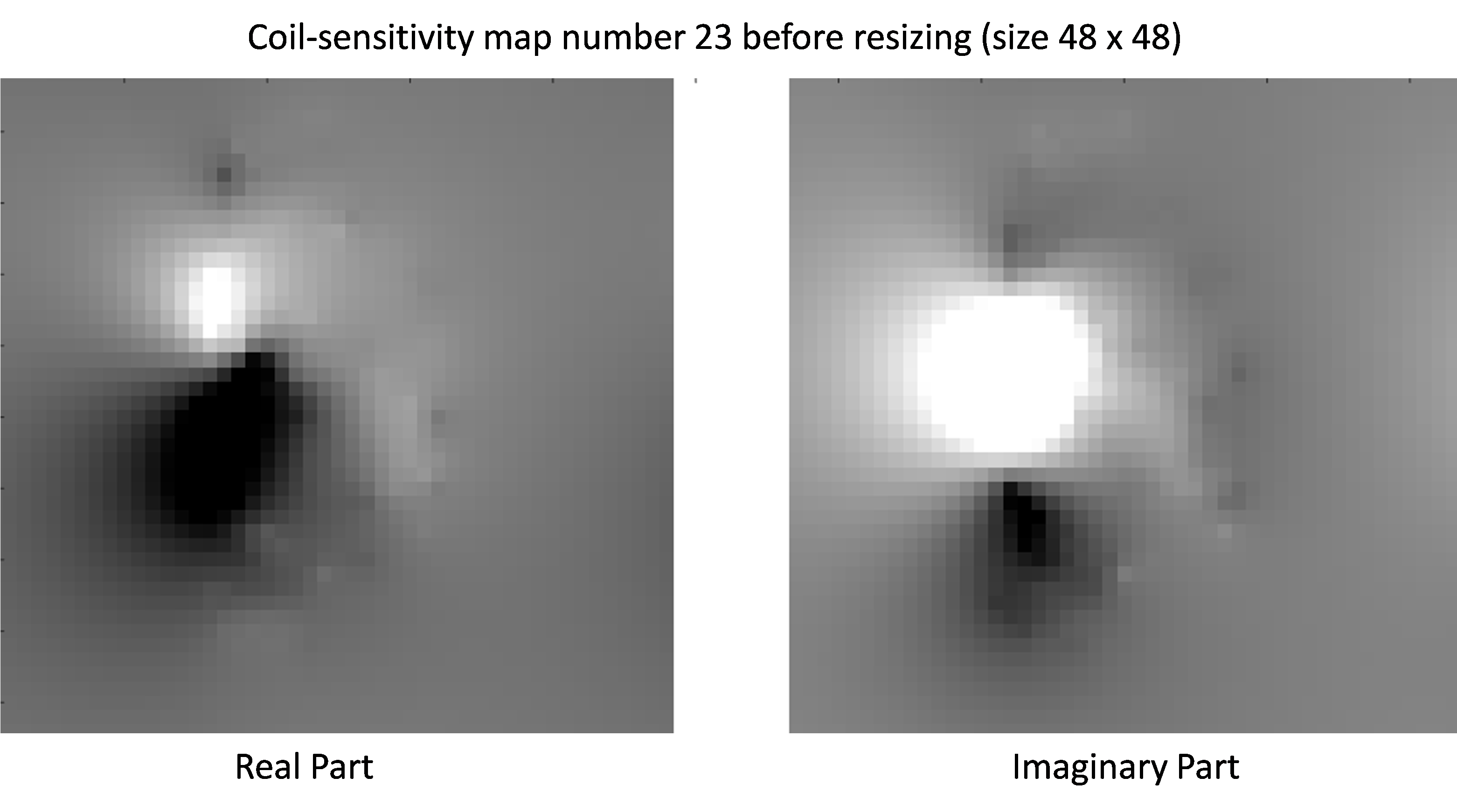
Resising the coil-sensitivity maps C is common in Monalisa since we usually estimate them with a low spatial resolution and frame-size, and we also store them with a small size to save disk-space and data-transfer time. Just before the reconstruction we resize then C to the frame-size as performed in the section above. For example, before resizing the coil-sensitivity numer 23 is of size 48 x 48 as in the following figure:
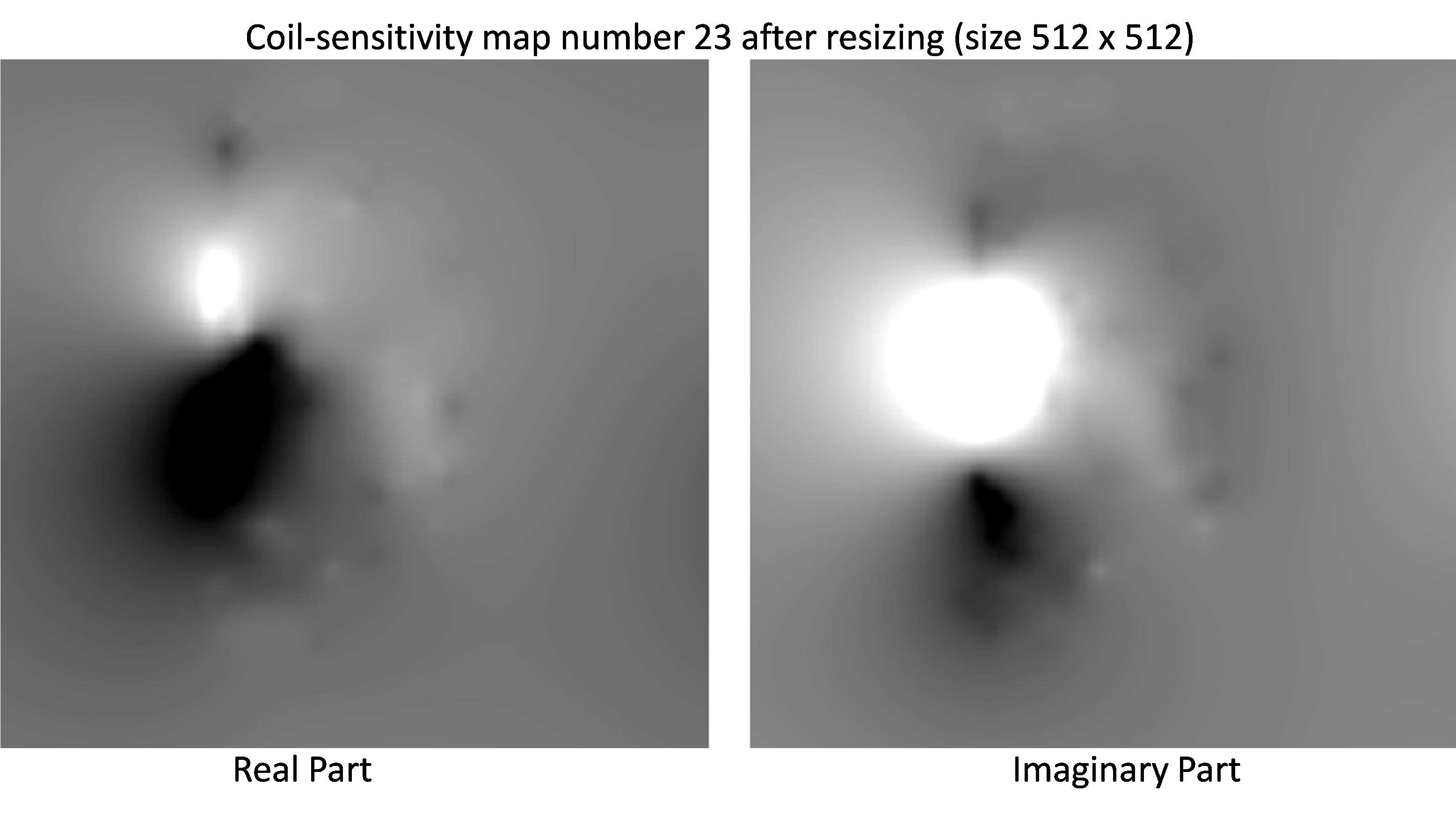
After resizing, the same coil-sensitivity map has the same size like the image we want to reconstruct (i.e. 512 x 512):
Evaluating the initial image for further iterative reconstructions
x0 = cell(nFr, 1);
for i = 1:nFr
    x0{i} = bmMathilda(y{i}, t{i}, ve{i}, C, N_u, N_u, dK_u);
end

bmImage(x0);
Left is the reconstructed image and right the ground-truth.
Evaluating gridding matrices
[Gu, Gut] = bmTraj2SparseMat(t, ve, N_u, dK_u);
\(l_1\)-regularized least-square reconstruction with 1 temporal dimension for non-cartesian data
Regularized least-square reconstruction with (non-motion-corrected) temporal \(l_1\)- regularization for non-cartesian data (TevaMorphosia_chain)
file_label      = 'tevaMorphosia_chain'; % label to name the file containing the result
frSize          = N_u;
nCGD            = 4;
nIter           = 30;

delta           = 0.5;
rho             = 10*delta;

regul_mode      = 'normal';

witness_ind = 1:5:nIter;
witnessInfo = bmWitnessInfo(file_label, witness_ind);


x = bmTevaMorphosia_chain(x0, ...
                        [], [], ...
                        y, ve, C, ...
                        Gu, Gut, frSize, ...
                        [], [], ...
                        delta, rho, regul_mode, ...
                        nCGD, ve_max, ...
                        nIter, witnessInfo);


bmImage(x)
Left is the reconstructed image and right the ground-truth.
Estimation of deformation fields
maxPixDisplacement  = 10;
nIter               = 500;
reg_file            = [];
reg_mask            = [];

h = x;
[DF_to_prev, imReg_to_prev]    = bmImDeformFieldChain_imRegDemons23(  h, frSize, 'curr_to_prev', nIter, 1, reg_file, reg_mask, maxPixDisplacement);
Evaluation of deformation matrices
[Tu, Tut] = bmImDeformField2SparseMat(DF_to_prev, N_u, [], true);
Regularized least-square reconstruction with motion-corrected temporal \(l_1\)- regularization for non-cartesian data (TevaMorphosia_chain)
file_label      = 'tevaMorphosia_chain_DF'; % label to name the file containing the result
frSize          = N_u;
nCGD            = 4;
nIter           = 30;

delta           = 1.5;
rho             = 10*delta;

regul_mode      = 'normal';

witness_ind = 1:5:nIter;
witnessInfo = bmWitnessInfo(file_label, witness_ind);


x = bmTevaMorphosia_chain(x0, ...
                        [], [], ...
                        y, ve, C, ...
                        Gu, Gut, frSize, ...
                        Tu, Tut, ...
                        delta, rho, regul_mode, ...
                        nCGD, ve_max, ...
                        nIter, witnessInfo);


bmImage(x)

Left is the reconstructed image and right the ground-truth.
Regularized least-square reconstruction with backward and forward (non-motion-corrected) temporal \(l_1\)- regularization for non-cartesian data (TevaDuoMorphosia_chain)
file_label      = 'tevaDuoMorphosia_chain'; % label to name the file containing the result
frSize          = N_u;
nCGD            = 4;
nIter           = 30;

delta           = 0.5;
rho             = 10*delta;

regul_mode      = 'normal';

witness_ind = 1:5:nIter;
witnessInfo = bmWitnessInfo(file_label, witness_ind);


x = bmTevaDuoMorphosia_chain(x0, ...
                            [], [], [], [], ...
                            y, ve, C, ...
                            Gu, Gut, frSize, ...
                            [], [], [], [], ...
                            delta, rho, regul_mode, ...
                            nCGD, ve_max, ...
                            nIter, witnessInfo);


bmImage(x)

Left is the reconstructed image and right the ground-truth.
Estimation of deformation fields
maxPixDisplacement  = 10;
nIter               = 500;
reg_file            = [];
reg_mask            = [];

h = x;
[DF_to_prev, imReg_to_prev]    = bmImDeformFieldChain_imRegDemons23(  h, frSize, 'curr_to_prev', nIter, 1, reg_file, reg_mask, maxPixDisplacement);
[DF_to_next, imReg_to_next]    = bmImDeformFieldChain_imRegDemons23(  h, frSize, 'curr_to_next', nIter, 1, reg_file, reg_mask, maxPixDisplacement);
Evaluating deformation matrices
[Tu1, Tu1t] = bmImDeformField2SparseMat(DF_to_prev, N_u, [], true);
[Tu2, Tu2t] = bmImDeformField2SparseMat(DF_to_next, N_u, [], true);
Regularized least-square reconstruction with backward and forward motion-corrected temporal \(l_1\)- regularization for non-cartesian data (TevaDuoMorphosia_chain)
file_label      = 'tevaDuoMorphosia_chain_DF'; % label to name the file containing the result
frSize          = N_u;
nCGD            = 4;
nIter           = 30;

delta           = 1.5;
rho             = 10*delta;

regul_mode      = 'normal';

witness_ind = 1:5:nIter;
witnessInfo = bmWitnessInfo(file_label, witness_ind);


x = bmTevaDuoMorphosia_chain(x0, ...
                            [], [], [], [], ...
                            y, ve, C, ...
                            Gu, Gut, frSize, ...
                            Tu1, Tu1t, Tu2, Tu2t, ...
                            delta, rho, regul_mode, ...
                            nCGD, ve_max, ...
                            nIter, witnessInfo);


bmImage(x)
Left is the reconstructed image and right the ground-truth.
\(l_2\)-regularized least-square reconstruction with 1 temporal dimension for non-cartesian data
Regularized least-square reconstruction with (non-motion-corrected) temporal \(l_2\)- regularization for non-cartesian data (SensitivaMorphosia_chain)
file_label      = 'sensitivaMorphosia_chain'; % label to name the file containing the result
frSize          = N_u;
nCGD            = 4;
nIter           = 30;

delta           = 5;

regul_mode      = 'normal';

witness_ind = 1:5:nIter;
witnessInfo = bmWitnessInfo(file_label, witness_ind);


x = bmSensitivaMorphosia_chain(  x0, ...
                                y, ve, C, ...
                                Gu, Gut, frSize, ...
                                [], [], ...
                                delta, regul_mode, ...
                                nCGD, ve_max, ...
                                nIter, witnessInfo  );


bmImage(x)
Left is the reconstructed image and right the ground-truth.
Estimation of deformation fields
maxPixDisplacement  = 10;
nIter               = 500;
reg_file            = [];
reg_mask            = [];

h = x;
[DF_to_prev, imReg_to_prev]    = bmImDeformFieldChain_imRegDemons23(  h, frSize, 'curr_to_prev', nIter, 1, reg_file, reg_mask, maxPixDisplacement);
Evalutation of deformation matrices
[Tu, Tut] = bmImDeformField2SparseMat(DF_to_prev, N_u, [], true);
Regularized least-square reconstruction with motion-corrected temporal \(l_2\)- regularization for non-cartesian data (SensitivaMorphosia_chain)
file_label      = 'sensitivaMorphosia_chain_DF'; % label to name the file containing the result
frSize          = N_u;
nCGD            = 4;
nIter           = 30;

delta           = 15;

regul_mode      = 'normal';

witness_ind = 1:5:nIter;
witnessInfo = bmWitnessInfo(file_label, witness_ind);


x = bmSensitivaMorphosia_chain(  x0, ...
                                y, ve, C, ...
                                Gu, Gut, frSize, ...
                                Tu, Tut, ...
                                delta, regul_mode, ...
                                nCGD, ve_max, ...
                                nIter, witnessInfo  );


bmImage(x)

Left is the reconstructed image and right the ground-truth.
Regularized least-square reconstruction with backward and forward (non-motion-corrected) temporal \(l_2\)- regularization for non-cartesian data (SensitivaDuoMorphosia_chain)
file_label      = 'sensitivaDuoMorphosia_chain'; % label to name the file containing the result
frSize          = N_u;
nCGD            = 4;
nIter           = 30;

delta           = 5;

regul_mode      = 'normal';

witness_ind = 1:5:nIter;
witnessInfo = bmWitnessInfo(file_label, witness_ind);


x = bmSensitivaDuoMorphosia_chain(  x0, ...
                                    y, ve, C, ...
                                    Gu, Gut, frSize, ...
                                    [], [], [], [], ...
                                    delta, regul_mode, ...
                                    nCGD, ve_max, ...
                                    nIter, witnessInfo  );


bmImage(x)
Left is the reconstructed image and right the ground-truth.
Estimation of deformation fields
maxPixDisplacement  = 10;
nIter               = 500;
reg_file            = [];
reg_mask            = [];

h = x;
[DF_to_prev, imReg_to_prev]    = bmImDeformFieldChain_imRegDemons23(  h, frSize, 'curr_to_prev', nIter, 1, reg_file, reg_mask, maxPixDisplacement);
[DF_to_next, imReg_to_next]    = bmImDeformFieldChain_imRegDemons23(  h, frSize, 'curr_to_next', nIter, 1, reg_file, reg_mask, maxPixDisplacement);
Evaluation of deformation matrices
[Tu1, Tu1t] = bmImDeformField2SparseMat(DF_to_prev, N_u, [], true);
[Tu2, Tu2t] = bmImDeformField2SparseMat(DF_to_next, N_u, [], true);
Regularized least-square reconstruction with backward and ofrward motion-corrected temporal \(l_2\)- regularization for non-cartesian data (SensitivaDuoMorphosia_chain)
file_label      = 'sensitivaDuoMorphosia_chain_DF'; % label to name the file containing the result
frSize          = N_u;
nCGD            = 4;
nIter           = 30;

delta           = 15;

regul_mode      = 'normal';

witness_ind = 1:5:nIter;
witnessInfo = bmWitnessInfo(file_label, witness_ind);


x = bmSensitivaDuoMorphosia_chain(  x0, ...
                                    y, ve, C, ...
                                    Gu, Gut, frSize, ...
                                    Tu1, Tu1t, Tu2, Tu2t, ...
                                    delta, regul_mode, ...
                                    nCGD, ve_max, ...
                                    nIter, witnessInfo  );


bmImage(x)

Left is the reconstructed image and right the ground-truth.
Further explanation
blablabla